


 ELK - Log Analytics
Applications
The Applications section is where you monitor the performance of your instrumented services with APM (application performance monitoring). Each one of your services reports its transactions, the operations it performs for its callers, and the spans inside them, such as database queries or calls to other services. From this data NetEye.Cloud derives the three indicators you’ll meet on almost every page of this section: latency (how long a service takes to respond), throughput (how many transactions it handles per minute) and failed transaction rate (the share of transactions that end in an error).
The section is organized the way an investigation usually goes:
Services lists all monitored services with their indicators. This is where you notice that something is wrong and pick the service to look at.
The Service overview is the page of a single service. It brings together its transactions, errors, dependencies, metrics and logs, so most of the troubleshooting happens here.
Traces lists the transactions collected across all services, ranked by how much they affect your users, and lets you follow a single request end to end.
Dependencies turns the view around and shows the databases, APIs and other external systems your services call, so you can tell whether a slowdown comes from your code, or from something it depends on.
Service Map draws all services and their connections, which helps you understand the architecture and see which services an issue could spread to.
All pages share the global time range and the environment selector, so when you move from one to another you will continue viewing the same data.
Roles and Permissions
The Applications views are read-only for all roles defined by the contract with your organization:
VIEWER: Read
EDITOR: Read
ADMIN: Read
Services
The service inventory is available under . The Inventory tab lists every service that has sent transactions or spans in the selected time range, with its environment, average latency, throughput and failed transaction rate, each with a sparkline of the last period. Click a column header to sort, for example by failed transaction rate to bring the least reliable services to the top, and use the Environment selector when you only want to see what’s in production.
The Comparison option adds a grey line to every sparkline showing the same indicator for an earlier period, such as the day or week before. This is what makes the inventory useful as a routine check: on a Monday morning, set the time range to the last 24 hours, compare with Week before, and then the services whose colored line sits visibly above the grey one will be the ones that became slower or less reliable over the weekend, without you having to remember what their normal values are.
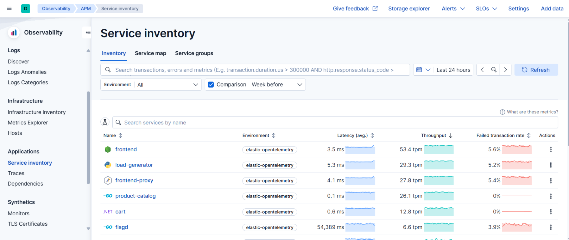
Clicking a service name opens its Service overview.
Note
A service appears in the inventory only if it has sent transactions or spans within the selected time range. Services that send only logs are not listed. If you expect a service and don’t see it, widen the time range first.
Service groups
When the inventory grows long, the Service groups tab lets you work with a subset. Each group is shown as a card with the number of services it contains and, if any, the number of active alerts on them, so a team can see the state of its own services without scrolling through everyone else’s.
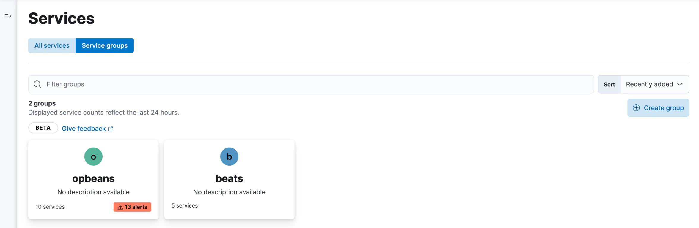
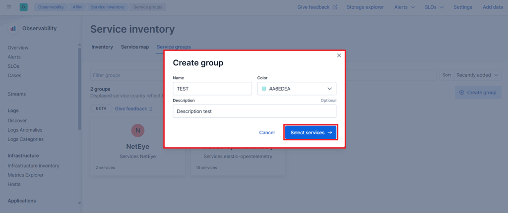
To create a group, click Create group, give it a name, a
color and optionally a description, then click
Select services and enter a query on the services’ attributes,
for example service.environment : "production" for all production
services or service.name : *beat for all services whose name ends in
beat. Services matching the query are assigned to the group
automatically, including ones that appear later.
Service Overview
The Service overview is the page of a single service and the place where most troubleshooting happens. Its tabs look at the same service from different angles and share the time range, environment and Comparison setting you select, so you can move between them without losing context.
Overview summarizes the health of the service: latency, throughput and failed transaction rate over time, the most frequent transactions, the most common errors and the dependencies it relies on. It also lists the service’s instances, that is, the individual processes or containers running it, each with its own latency, throughput and failed transaction rate, plus its CPU and memory usage. When the service as a whole looks fine but a small number of users are complaining, this table is where you might find out that one instance out of five is at 99% memory and responding slowly.

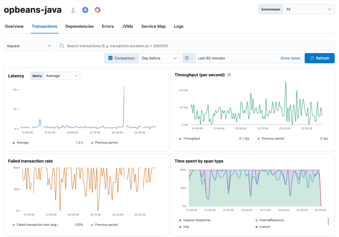
Transactions lists the operations the service performs, such as the endpoints of an API or the jobs of a worker, each with its own latency, throughput and failed transaction rate, and shows four charts for the selected transaction type: latency, throughput, failed transaction rate and time spent by span type. The last one splits the latency into what the service did itself and what it spent waiting on HTTP calls, database queries and so on.
Suppose the checkout service has become slow. Here you can see that the latency chart has a single sharp spike at 22:20 rather than a gradual rise, that throughput didn’t change at that moment, and from the span type breakdown whether the extra time went into the application code or into external calls. That already tells you whether to look at a deployment, at a dependency or at the service’s own resources.
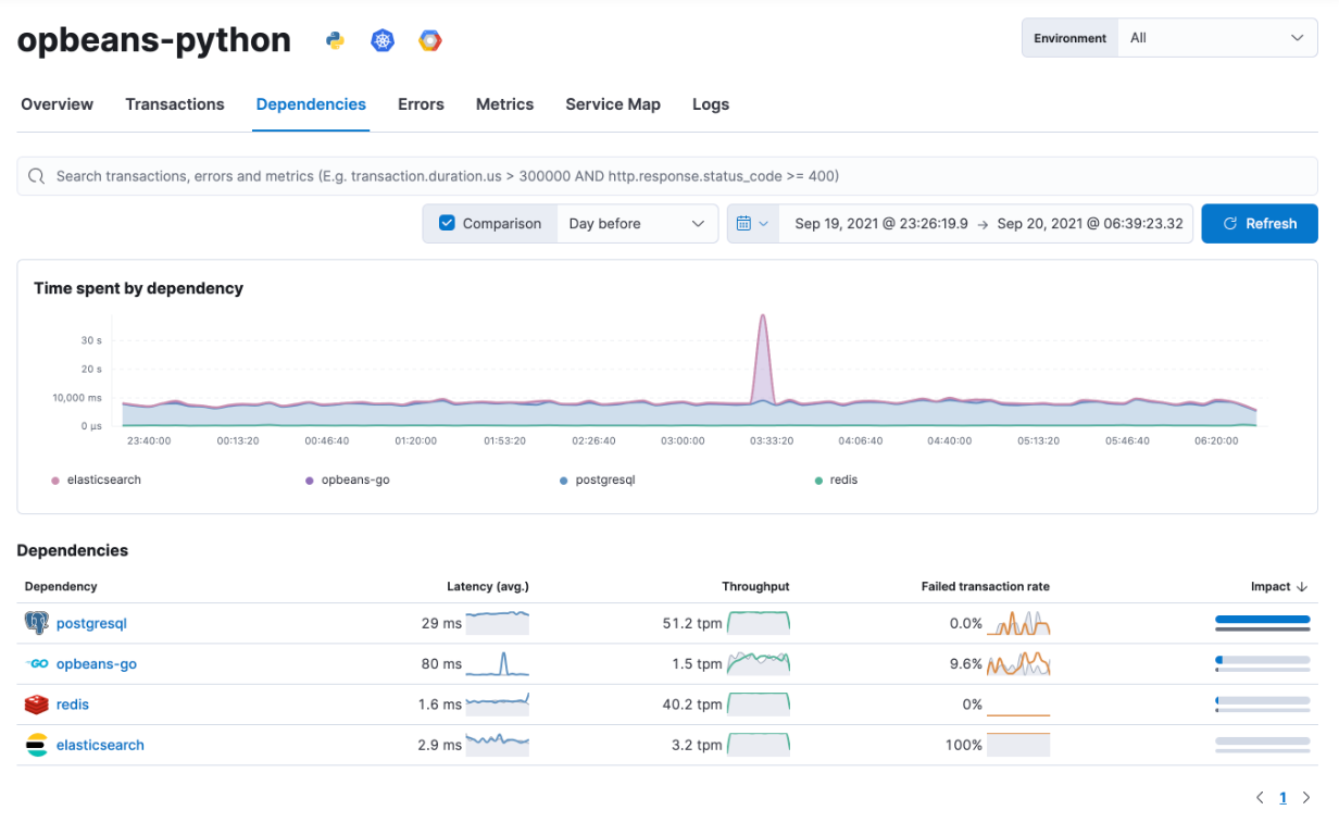
Dependencies shows the external systems and downstream services this service calls, with a chart of the time spent in each dependency and a table ranking them by impact. Continuing the example: if the span type breakdown pointed to external calls, this chart shows which dependency produced the spike. A single dependency peaking while the others stay flat tells you the problem is in that database or downstream service, not in the service you started from.
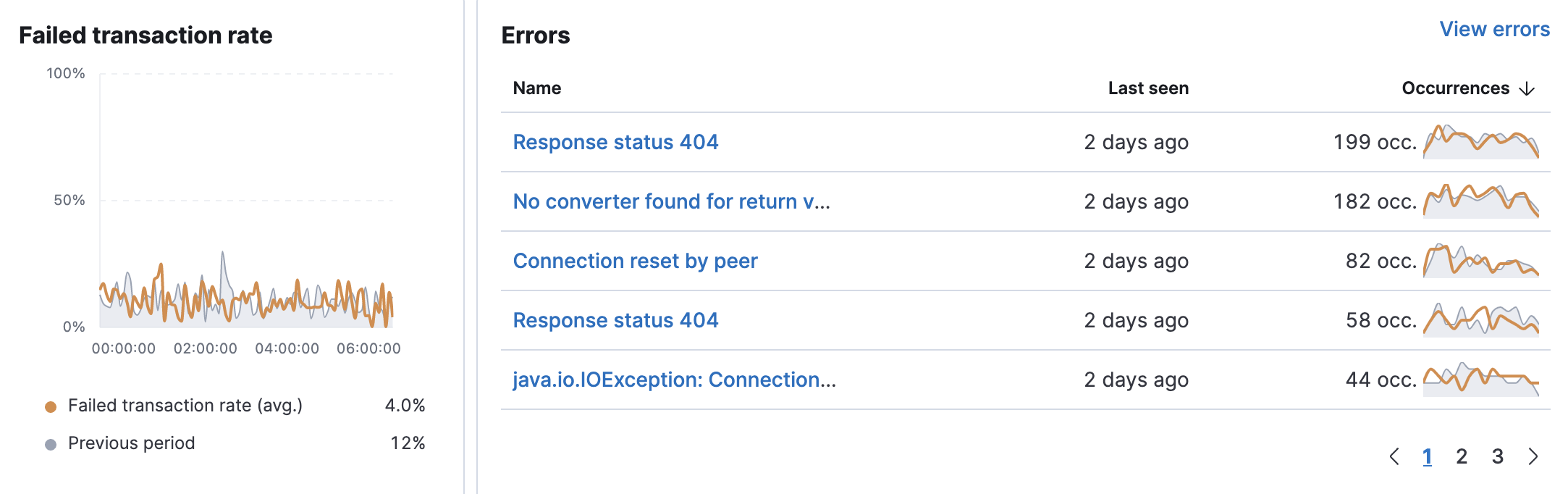
Errors groups the errors captured for the service by type and message, such as when each was last seen and how often it occurred, next to the failed transaction rate over time. Open a group to see a sample occurrence with its stack trace and the transaction it happened in. The occurrence counts are the quickest way to tell the difference between a new error that appeared in the last release and a known one that has been there for months.
Metrics (named JVMs for Java services) shows the resource consumption of the service’s runtime, such as CPU, memory and garbage collection, as reported by the APM agent. Use it when you suspect that the service itself, rather than a dependency, is running out of resources.
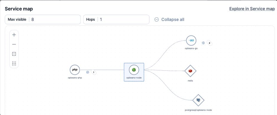
Service Map shows this service in the middle, with the services that call it on the left, and the services and systems it calls on the right. Use Hops to follow the connections further and Max visible to limit the number of nodes; click Explore in Service map to open the full map centered on this service, as described in Service Map.
Logs shows the log entries written by the service in the selected time range, so without leaving the page you can read what the application reported at the moment a transaction was slow or failed.
Traces
A trace is the record of a single request as it travels through your services: the transaction that received it, the spans it executed and the transactions it triggered in other services, each with its duration and outcome. Traces lists the transactions collected across all services in the selected time range, so you can go from an aggregated indicator to one concrete request and see precisely what happened.
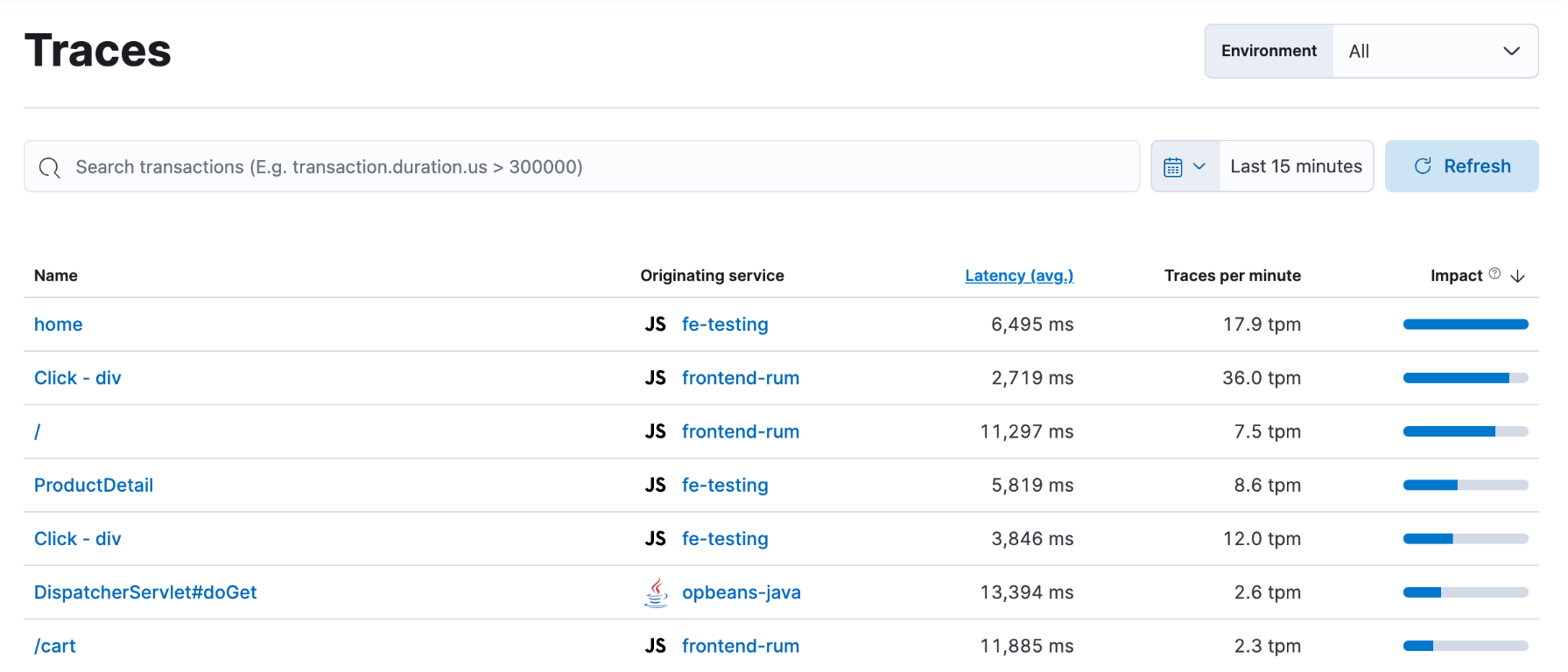
Each row shows the transaction name, the service it originated in, its average latency, how many traces per minute it produces and its impact. Impact is latency multiplied by throughput: a transaction that is both slow and frequently called has a high impact, while a slow one that is rarely called, or a fast one that is called constantly, ranks lower.
The list is sorted by impact by default, which puts the transactions whose optimization would benefit users most at the top. This is the list to start from when you have a performance budget and need to decide what to work on first, rather than when you’re chasing a specific incident.
Click a transaction to open its trace: a timeline of every span in the order it ran, nested under the span that called it, with the service each span belongs to, its duration and any error it produced. Reading it from top to bottom takes you to the step responsible for the latency or the failure, even when that step ran in a different service from the one where the symptom appeared.
Dependencies
Dependencies is where you analyze the external systems and downstream services your applications depend on. Whereas the Services inventory shows the services you run, this view shows what they call: databases, caches, message queues, external APIs and other backend components, all in one list regardless of which service is calling them.
Open . The table lists each dependency with the average latency, throughput and failed transaction rate of the calls made to it, along with its impact. Next to each value a sparkline, a small inline chart, shows how the metric evolved over the selected time range; the Comparison option adds a grey line to each sparkline showing the previous period, as in the Services inventory. Click a column header to sort, and a dependency name to see which services call it.
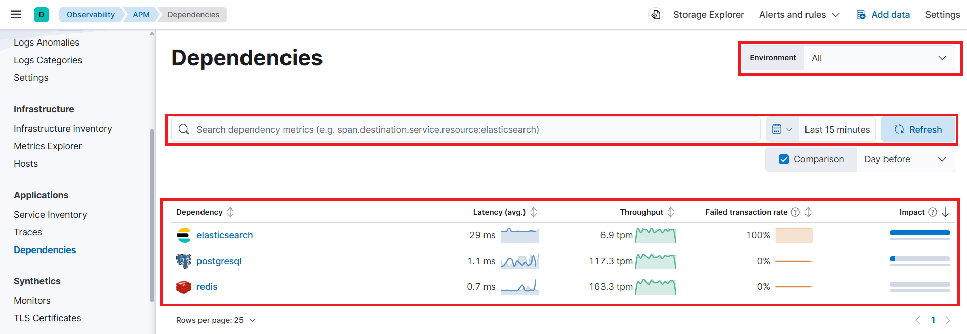
For each dependency you can:
See who calls it and how it performs. Latency, throughput and failed transaction rate of the calls made to it, and the services that make them.
Measure its impact. How much of your services’ total time is spent waiting for this dependency. The table is sorted by impact by default, so the systems that cost you the most response time are at the top.
Find out whose fault it is. If a database or API is slow for all its callers, the problem is likely on the external side; if only one service suffers, it’s more likely how that service is using it.
Discover what you’re calling. The list shows every external system your applications actually talk to, including ones you may not expect, such as a third-party API still used by an old module.
Example: three unrelated services all show higher latency one morning. Checked one by one they have nothing in common; sorted by impact on this page, a single Postgres instance sits at the top with three times its usual latency, and all three services turn out to be among its callers.
Note
If a dependency isn’t an instrumented service of yours, this is the only place where its behavior becomes visible at all.
Service Map
The Service Map, reached from the Service map tab of the service inventory, draws a graph of all instrumented services in the selected environment and the connections between them as observed in the traces: if service A called service B, there is a line from A to B. Databases, caches and external hosts appear as well, so the map shows the whole path a request can take.
Use it to get the picture of an architecture you’re not familiar with, or to answer questions that are hard to answer from lists: which services are affected if this database is slow, which service sits in the middle of most request paths, and whether a connection exists that shouldn’t. Click a node to open the Service overview of that service, and use the environment selector and the search bar to reduce the map to the part you care about.
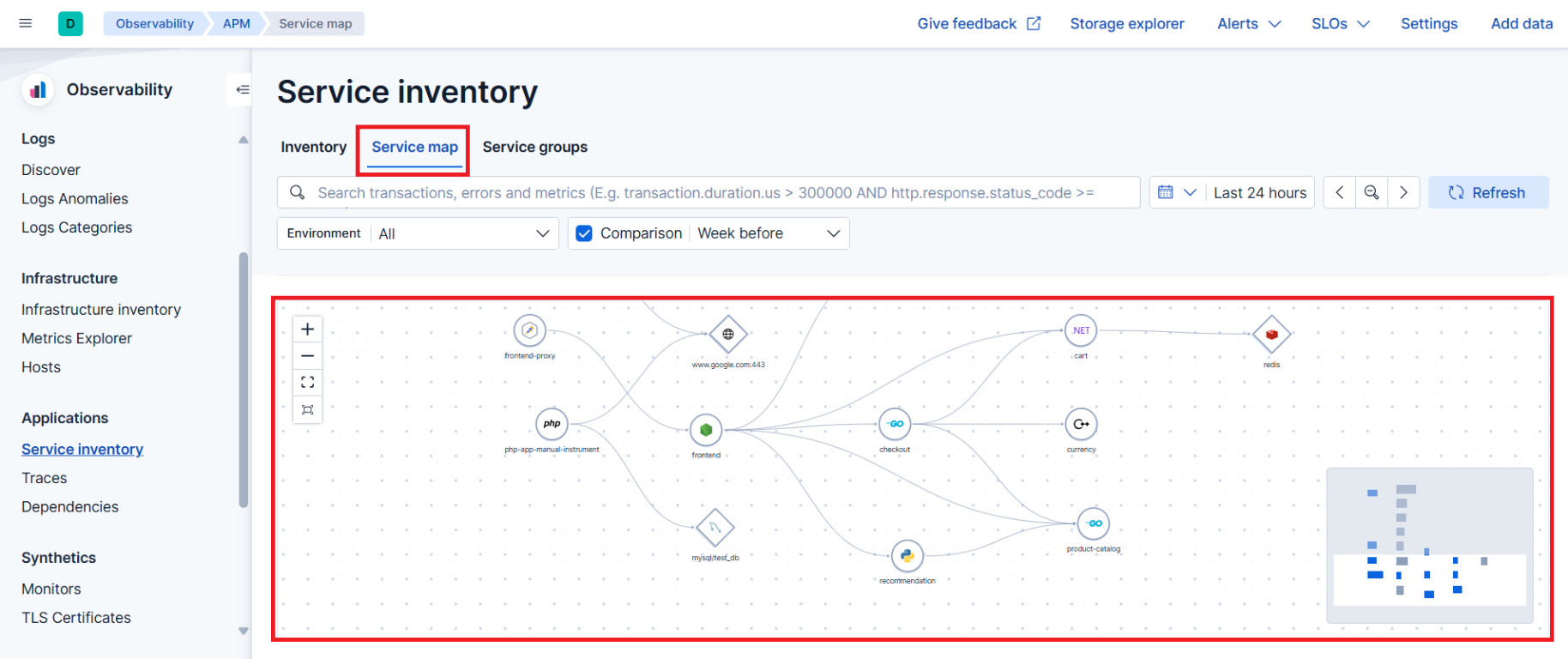
The map is built from distributed traces. A service that isn’t instrumented, or doesn’t propagate the trace context, appears without connections or not at all.

